scale.olm.core

The scale.olm.core module contains classes that have a core capability that could be used by any component of OLM and even on their own outside of OLM. Maybe one day they will become their own package as scale-core instead of scale-olm-core. Here are some principles for the core.

• The core should only contain classes.

• Each class should have doctests demonstrating the happy path, i.e. not errors or edge cases.

• The unit tests for a core class are at testing/core_ClassName.test.py file and should address edge cases and other behavior.

• Classes can be further demonstrated in notebooks, notebooks/core_ClassName_demo.ipynb.

class ArpInfo

Handle the ARPDATA.TXT format for ORIGEN reactor libraries.

create_temp_archive(arpdata_txt, temp_arc)

Create a temporary HDF5 archive file from an arpdata.txt.

get_arpdata()

Return the arpdata.txt file block for this data.

get_dim_by_index(i)

Get the dimension tuple from the flat index.

get_dims()

Get the total dimension size.

get_index_by_dim(dim)

Get the flat index by a dimensional tuple.

get_lib_by_index(i)

Get the library by flat index.

get_perm_by_index(i)

Get the original permutation index that created this ARP point in space by flat index of libraries.

get_space()

Get the dictionary that describes this point in space.

init_block(name, block)

Initialize data from a single block of arpdata WITHOUT the ! line

init_mox(name, lib_list, pu239_frac_list, pu_frac_list, mod_dens_list)

Initialize MOX data for arpdata.txt format from a list of data.

init_uox(name, lib_list, enrichment_list, mod_dens_list)

Initialize UOX data for arpdata.txt format from a list of data.

interptags_by_index(i)

Get the interpolation tags from the flat index.

interpvars_by_index(i)

Get the interpolation variables from the flat index.

num_libs()

Get the total number of libraries.

static parse_arpdata(file)

Simple function to parse the blocks of arpdata.txt

restrict(axis_name, keep_values)

Restrict values on the axis.

Returns a new arpinfo object.

Note that it does not modify the libraries themselves! So burnups must be modified in place on the libraries outside this function.

class BurnupHistory(time, burnup, epsilon_dbu: float = 0.0)

Manages a time versus burnup power history.

Parameters:

• time – List of cumulative times, monotonically strictly increasing, each time must be greater than the last.

• burnup – list of cumulative burnups, monotonically increasing, each burup must be greater or equal to the last.

• epsilon_dbu – The small value of burnup changes to disregard (default: 0), can be useful for avoiding tiny numerical precision issues when the input burnups are subtracted.

classify_operations(min_shutdown_time: float = 0.0, min_shutdown_power: float = 0.0, starts_within_cycle: int = None)

Classify the operating history into cycles, downtime, etc.

The output of this function is a dictionary of information that can be used to classify the operating history into cycles. By default we consider that any time with zero power is a shutdown and thus starts a new cycle.

Here is an example of the dictionary returned.

time =   [0, 5,  10,  50,  55,  100,  105]
burnup = [0, 0, 100, 500, 500, 1000, 1000]
bh = BurnupHistory(time, burnup)
x = bh.classify_operations()

{
    "options": {
        "min_shutdown_time": 0.0,
        "min_shutdown_power": 0.0,
        "starts_within_cycle": null
    },
    "operations": [
        {
            "cycle": "",
            "within_cycle": false,
            "start": 0,
            "end": 1
        },
        {
            "cycle": "1",
            "within_cycle": true,
            "start": 1,
            "end": 3
        },
        {
            "cycle": "",
            "within_cycle": false,
            "start": 3,
            "end": 4
        },
        {
            "cycle": "2",
            "within_cycle": true,
            "start": 4,
            "end": 5
        },
        {
            "cycle": "",
            "within_cycle": false,
            "start": 5,
            "end": 6
        }
    ]
}

Parameters:

• min_shutdown_time – Minimum time to consider as a shutdown.

• min_shutdown_power – Minimum power to consider as a shutdown.

• starts_within_cycle – Instead of starting with cycle 1, start with this.

Returns:

A list of dictionaries described above.

Return type:

list[dict]

Examples

Create a simple operating history. Our numbers can be interpreted to be in days and MWd/MTU for time and burnup respectively.

>>> time =   [0, 5,  10,  50,  55,  100,  105]
>>> burnup = [0, 0, 100, 500, 500, 1000, 1000]
>>> bh = BurnupHistory(time, burnup)

The time for each interval is calculated.

>>> bh.interval_time
[5, 5, 40, 5, 45, 5]

The power for each interval is calculated as burnup/time.

>>> bh.interval_power
[0.0, 20.0, 10.0, 0.0, 11.11111111111111, 0.0]

We will classify operations on this operating history to demonstrate that the defaults will result in the short 5 days of zero power being considered part of the cycle.

>>> x = bh.classify_operations()

Let’s create a function to print the information.

>>> def print_classification(x):
...     print(x['options'])
...     for op in x['operations']:
...         msg = 'during cycle ' + op['cycle'] if op['within_cycle'] else 'shutdown'
...         for i in range(op['start'],op['end']):
...             print("interval {} is {} with power {:.4g} MW/MTU for {:.4g} days".format(
...                 i,
...                 msg,
...                 bh.interval_power[i],
...                 bh.interval_time[i])
...             )
>>> print_classification(x)
{'min_shutdown_time': 0.0, 'min_shutdown_power': 0.0, 'starts_within_cycle': None}
interval 0 is shutdown with power 0 MW/MTU for 5 days
interval 1 is during cycle 1 with power 20 MW/MTU for 5 days
interval 2 is during cycle 1 with power 10 MW/MTU for 40 days
interval 3 is shutdown with power 0 MW/MTU for 5 days
interval 4 is during cycle 2 with power 11.11 MW/MTU for 45 days
interval 5 is shutdown with power 0 MW/MTU for 5 days

Now let’s classify again but with a minimum shutdown time of 10 days so that the intra-cycle power dip does not appear as a reload and we just have one cycle.

>>> x = bh.classify_operations(min_shutdown_time=10.0)
>>> print_classification(x)
{'min_shutdown_time': 10.0, 'min_shutdown_power': 0.0, 'starts_within_cycle': None}
interval 0 is shutdown with power 0 MW/MTU for 5 days
interval 1 is during cycle 1 with power 20 MW/MTU for 5 days
interval 2 is during cycle 1 with power 10 MW/MTU for 40 days
interval 3 is during cycle 1 with power 0 MW/MTU for 5 days
interval 4 is during cycle 1 with power 11.11 MW/MTU for 45 days
interval 5 is shutdown with power 0 MW/MTU for 5 days

get_cycle_time(x)

Return a new time array for each cycle from the output of classify_operations.

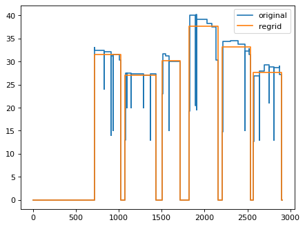
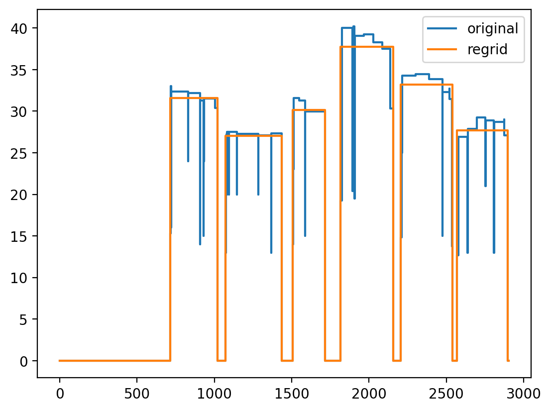
One way this class is useful is to pass into the regrid function, which takes a list of (cumulative) times.

import matplotlib.pyplot as plt
from scale.olm.core import BurnupHistory

time0,burnup0 = BurnupHistory._testing_data_sfcompo1()
bh = BurnupHistory(time0, burnup0)

bh.plot_power_history(label='original')

x = bh.classify_operations(min_shutdown_time=10.0)
new_time = bh.get_cycle_time(x)

bh2 = bh.regrid(new_time)
bh2.plot_power_history(label='regrid', add_to_existing=True)

plt.legend()
plt.show()

(png, hires.png, pdf)

Using get_cycle_time to determine cycle-average powers.

plot_power_history(label=None, add_to_existing=False, **kwargs)

Return a plot of the power in each interval.

regrid(time, burnup_interp=None)

Project to a new time grid.

static union_times(a, b, kind='mergesort')

Union two time grids and sort properly.

class CompositionManager(data)

Stores the basic nuclide data and provides calculations.

Parameters:

data – The basic data in ii.json-style format.

data

nuclide data

Type:

dict

Examples:

Initialize with fake data.

>>> data = {
...     "0001001": {
...         "IZZZAAA": "0001001",
...         "atomicNumber": 1,
...         "element": "H",
...         "isomericState": 0,
...         "mass": 1.007830023765564,
...         "massNumber": 1
...     },
...     "0001002": {
...         "IZZZAAA": "0001002",
...         "atomicNumber": 1,
...         "element": "H",
...         "isomericState": 0,
...         "mass": 2.0141000747680664,
...         "massNumber": 2
...     }
... }
>>> cm = CompositionManager(data)

Output the mass.

>>> cm.mass("h2")
2.0141000747680664

Do name conversions.

>>> cm.eam("0001002")
'h2'
>>> cm.eam("h2")
'h2'
>>> cm.izzzaaa("h2")
'0001002'

static approximate_hm_info(comp)

Approximate some heavy metal information.

static calculate_hm_oxide_breakdown(x)

Calculate the oxide breakdown from weight percentages in x for all heavy metal.

eam(id: str) → str

Return an eam like ‘am242m’ from either an eam or izzzaaa identifier.

Parameters:

id – The identifier either an eam or izzzaaa like ‘1095242’.

Returns:

An eam nuclide identifier.

Return type:

str

static form_eam_from_eai(e: str, a: int, i: int) → str

Form an eam identifier from e,a,i triplet.

static form_izzzaaa(i: int, z: int, a: int) → str

Form an izzzaaa identifier from i,z,a triplet.

static grams_per_mol(iso_wts: dict[str, float], m_data: dict[str, float] = {'am241': 241.0568}) → float

Calculate the grams per mole of a mass fraction mixture.

Use the formula to calculate the total mixture molar mass \(m\) according to

\[ \begin{align}\begin{aligned}1/m = \sum_i w_i / m_i\\\sum_i w_i = 1.0\end{aligned}\end{align} \]

for each nuclide \(i\).

The values for the individual molar masses are \(m_i\) are provided in the m_data dict. This is not very important for the purposes of this code that these values be precise. If not present in the dict, the simple mass number is used, i.e. 242 for am242m.

Parameters:

• iso_wts – Dictionary with keys as nuclide names (e.g. ‘am241’) and values proportional to mass fraction.

• m_data – Optional molar masses (grams/mol).

Returns:

The total molar mass m from the above formula.

Examples

Force the use of mass numbers by providing empty mass data

>>> CompositionManager.grams_per_mol({'u235': 50, 'pu239': 50}, m_data={})
236.9831223628692

izzzaaa(id: str) → str

Return an izzzaaa like ‘1095242’ from either an eam or izzzaaa identifier.

Parameters:

id – The identifier either an eam like ‘am242m’ or izzzaaa.

Returns:

An izzzaaa nuclide identifier.

Return type:

str

mass(id: str, default: float = None) → float

Return the mass for a specific nuclide.

static parse_eam_to_eai(id: str)

Parse an eam nuclide identifier into an e,a,i tuple.

static parse_izzzaaa(id: str)

Parse an izzzaaa nuclide identifier into an i,z,a triplet.

static renormalize_wtpt(wtpt0, sum0, key_filter='')

Renormalize to sum0 any keys matching filter.

class FileHasher(file: Path)

Hashes the content of a file.

Parameters:

file – Path to an existing file.

id

Hash of the contents of the file.

Type:

str

Examples

>>> from scale.olm.core import TempDir
>>> td = TempDir()
>>> a_path = td.write_file("some duplicate content","a.txt")
>>> b_path = td.write_file("some duplicate content","b.txt")
>>> FileHasher(a_path).id
'161da18e656052f506f6283f71168d6a'
>>> FileHasher(b_path).id
'161da18e656052f506f6283f71168d6a'

class InventoryInterface(input)

Loads/saves and extracts data from the inventory interface file.

class NuclideInventory(composition_manager, time, nuclide_amount, time_units='SECONDS', amount_units='MOLES')

Manages a time-dependent nuclide inventory.

get_nuclides(nice_label=False)

Return the nuclides in this system

rel_diff(nuclide, other_self, units='GRAMS', eps=1e-12)

Create a relative difference.

wrel_diff(nuclide, other_self, units='GRAMS')

Create a weighted relative difference.

class Obiwan(obiwan)

Wrap obiwan.

static get_history_from_f71(obiwan, f71, caseid0)

Parse the history of the form as follows for 6.3 series:

pos         time        power         flux      fluence       energy    initialhm libpos   case   step DCGNAB
(-)          (s)         (MW)    (n/cm2-s)      (n/cm2)        (MWd)      (MTIHM)    (-)    (-)    (-)    (-)
  1  0.00000e+00  4.00000e+01  8.11143e+14  0.00000e+00  0.00000e+00  1.00000e+00      1      1      0 DC----
  2  2.16000e+06  4.00000e+01  6.22529e+14  1.53582e+21  1.00000e+03  1.00000e+00      1      1     10 DC----
  3  2.16000e+07  4.00000e+01  4.26681e+14  8.78948e+21  1.00000e+04  1.00000e+00      2      1     10 DC----
  4  5.40000e+07  4.00000e+01  4.26566e+14  1.34274e+22  2.50000e+04  1.00000e+00      3      1     10 DC----
  5  1.08000e+08  4.00000e+01  4.31263e+14  2.30677e+22  5.00000e+04  1.00000e+00      4      1     10 DC----
  6  1.51200e+08  4.00000e+01  4.32303e+14  1.86058e+22  7.00000e+04  1.00000e+00      5      1     10 DC----
  7  1.94400e+08  4.00000e+01  4.33742e+14  1.86669e+22  9.00000e+04  1.00000e+00      6      1     10 DC----
  8  2.37600e+08  4.00000e+01  4.35733e+14  1.87415e+22  1.10000e+05  1.00000e+00      7      1     10 DC----

Parse the history of the form as follows for 7.0 series:

pos         time        power         flux      fluence       energy    initialhm       volume libpos   case   step DCGNAB
(-)          (s)         (MW)   (n/cm^2-s)     (n/cm^2)        (MWd)      (MTIHM)       (cm^3)    (-)    (-)    (-)    (-)
  1  0.00000e+00  0.00000e+00  0.00000e+00  0.00000e+00  0.00000e+00  1.00000e+00  1.09091e+05      1     10      0 DC----
  2  2.16000e+06  3.99302e+01  2.77611e+14  5.99639e+20  9.98255e+02  1.00000e+00  1.09091e+05      2     10      1 DC----
  3  2.16000e+07  3.99294e+01  2.88762e+14  6.21316e+21  9.98238e+03  1.00000e+00  1.09091e+05      3     10      2 DC----
  4  5.40000e+07  3.99271e+01  3.13691e+14  1.63767e+22  2.49551e+04  1.00000e+00  1.09091e+05      4     10      3 DC----
  5  8.10000e+07  3.99215e+01  3.42857e+14  2.56339e+22  3.74305e+04  1.00000e+00  1.09091e+05      5     10      4 DC----
  6  1.08000e+08  3.99155e+01  3.70174e+14  3.56286e+22  4.99041e+04  1.00000e+00  1.09091e+05      6     10      5 DC----
  7  1.29600e+08  3.99087e+01  3.95311e+14  4.41673e+22  5.98813e+04  1.00000e+00  1.09091e+05      7     10      6 DC----
  8  1.51200e+08  3.99026e+01  4.18116e+14  5.31986e+22  6.98569e+04  1.00000e+00  1.09091e+05      8     10      7 DC----

class ReactorLibrary(file, name='', progress_bar=True)

Simple class to read an ORIGEN ReactorLibrary into memory. The hierarchy of ORIGEN data is a Transition Matrix is the necessary computational piece. A Library is a time-dependent sequence of Transition Matrices. A ReactorLibrary is a multi-dimensional interpolatable space of Libraries.

static duplicate_degenerate_axis_value(x0)

Create a second axis value for degenerate axes to enable gradient calculations.

When an axis has only one value, numpy.gradient cannot compute gradients. This function creates a second value with positive spacing from the original.

Parameters:

x0 – The original axis value

Returns:

The second axis value (x1) such that x1 > x0

Examples

>>> ReactorLibrary.duplicate_degenerate_axis_value(0.723)
0.773
>>> ReactorLibrary.duplicate_degenerate_axis_value(-1.0)
-0.95
>>> ReactorLibrary.duplicate_degenerate_axis_value(0.0)
0.05
>>> ReactorLibrary.duplicate_degenerate_axis_value(100.0)
105.0

restrict(axis_name, keep_values)

Restrict the data set returning a new one.

class ScaleOutfile(outfile: str)

Extracts basic information from a SCALE main output file.

Parameters:

outfile (str) – The path to the SCALE output file.

Examples

>>> info = ScaleOutfile(scale_outfile)
>>> info.outfile == scale_outfile
True
>>> info.version
'6.3.0'
>>> len(info.sequence_list)
1
>>> s0 = info.sequence_list[0]
>>> s0['sequence']
't-depl'
>>> s0['product']
'TRITON'
>>> s0['runtime_seconds']
35.2481

outfile

The path to the SCALE .out file.

Type:

str

sequence_list

Information extracted for each sequence in order - sequence (str) - runtime_seconds (float) - product (str)

Type:

list[dict]

Initializes the ScaleOutfile instance.

Parameters:

outfile (str) – The path to the SCALE output file.

Examples:

>>> info = ScaleOutfile(scale_outfile)
>>> info.version
'6.3.0'

static get_product_name(sequence: str) → str

Maps the sequence information to a product name.

Parameters:

sequence – sequence name.

Returns:

Corresponding product name.

Examples

>>> ScaleOutfile.get_product_name('t-depl-1d')
'TRITON'

static parse_burnups_from_triton_output(output)

Parse the table that looks like this:

Sub-Interval   Depletion   Sub-interval    Specific      Burn Length  Decay Length   Library Burnup
     No.       Interval     in interval  Power(MW/MTIHM)     (d)          (d)           (MWd/MTIHM)
----------------------------------------------------------------------------------------------------
----------------------------------------------------------------------------------------------------
        0     ****Initial Bootstrap Calculation****                                      0.00000E+00
        1          1                1          40.000      25.000         0.000          5.00000e+02
        2          1                2          40.000     300.000         0.000          7.00000e+03
        3          1                3          40.000     300.000         0.000          1.90000e+04
        4          1                4          40.000     312.500         0.000          3.12500e+04
        5          1                5          40.000     312.500         0.000          4.37500e+04
        6          1                6          40.000     333.333         0.000          5.66667e+04
        7          1                7          40.000     333.333         0.000          7.00000e+04
        8          1                8          40.000     333.333         0.000          8.33333e+04
----------------------------------------------------------------------------------------------------

class ScaleRunner(scalerte_path: Path, do_not_run: bool = None)

A basic wrapper class around SCALE Runtime Environment (scalerte).

Initialize and check the runtime for various key quantities.

Parameters:

scalerte_path – The path to the runtime, e.g. /my/install/bin/scalerte

Examples:

runner = ScaleRunner('/my/install/bin/scalerte')
runner.version
runner.run('/path/to/scale.inp')

scalerte_path`

The path to the scalerte executable.

args

Arguments to use when invoking SCALE (see set_args)

version

The version of the SCALE Runtime Environment.

data_dir

The path to the SCALE data directory.

data_size

The size of the SCALE data directory.

run(input_file)

Run an input file through SCALE.

Verify first that the file was not already successfully run.

Parameters:

• input_file – path to the input file

• args – arguments

Raises:

• ValueError – If the input file does not exist.

• ValueError – If the SCALE data directory does not exist.

Returns:

path to input_file as pssed in dict[str,]: dictionary of arbitrary runtime data to pass out to the user

Return type:

str

set_args(args)

Set the arguments to use for subsequent run calls.

Parameters:

args (str) – arguments as a single string

class TempDir

Creates a temporary directory that self-deletes.

Deletes the directory when the class goes out of scope.

Examples

Create a temporary directory.

>>> from scale.olm.core import TempDir
>>> td = TempDir()
>>> path = td.path
>>> path.exists() and path.is_dir()
True

When the object goes out of scope, the directory is deleted.

>>> td = None
>>> path.exists()
False

path

path to the temporary directory

write_file(text: str, name: str) → Path

Write text to a file name in the temporary directory.

Parameters:

• text – Text to write.

• name – Name of the file to write to in the temp directory.

Returns:

Filename that was created.

Examples

Create a file.

>>> td = TempDir()
>>> file = td.write_file("CONTENT","my.txt")
>>> file.name
'my.txt'
>>> file.parent == td.path
True

class TemplateManager(paths=[], include_env=True)

Manage jinja templates.

Finds all jinja templates in provided paths, including the local “templates” path inside OLM and the OLM_TEMPLATES_PATH environment variable.

Paths are searched in order starting with those provided to init, then the OLM_TEMPLATES_PATH then the local.

Templates MUST have a double extension like my.jt.inp with .jt. to be recognized.

Parameters:

list[str] (paths) – additional user paths to search

templates dict[str,pathlib.Path]

dict of all available template names, paths

paths list[str]

list of paths that were searched (including local and environment)

Examples:

Create a temporary directory and write two template files to it.

>>> td = TempDir()
>>> path1 = td.write_file("Hello {{noun}}.","line1.jt.inp")
>>> subdir = td.path / 'y' / 'z'
>>> subdir.mkdir(parents=True)
>>> path2 = td.write_file("Is there {{noun}} out there?","y/z/line2.jt.inp")

Create a template manager which will find those paths.

>>> tm = TemplateManager(paths=[td.path], include_env=False)
>>> tm.names()
['line1.jt.inp', 'y/z/line2.jt.inp']

>>> tm.expand('line1.jt.inp',{"noun":"hello"})
'Hello hello.'

>>> tm.expand('y/z/line2.jt.inp',{"noun":"anybody"})
'Is there anybody out there?'

expand(name: str, data: dict)

Expand a template by name using provided data.

Parameters:

• name – template name

• data – dictionary with all the data

Returns:

text from the expanded template and data

Return type:

str

static expand_file(path: Path, data: dict)

Returns expanded text from a file.

Parameters:

• path – path containing a file to read

• data – dictionary containing data

Returns:

expanded text

Return type:

str

static expand_text(text: str, data: dict, src_path: str = '')

Returns the expanded text with data.

Use jinja to expand the text with data.

Parameters:

• text – text containing jinja directives

• data – dictionary containing data

Raises:

ValueError – if jinja raises an undefined variable error

Returns:

expanded text

Return type:

str

names()

Return the names of all the templates.

Returns:

names of templates

Return type:

list[str]

path(name: str)

Return a template file by name.

Parameters:

name – template name

Returns:

full path to the template

Return type:

str

class ThreadPoolExecutor(max_workers: int = 2, progress_bar: bool = True)

Executes in parallel using threads.

Parameters:

• max_workers – Number of parallel workers to use.

• progress_bar – If progress bar output should be enabled–it can be useful to disable for tests and other non-interactive use cases.

Examples

>>> from scale.olm.core import ThreadPoolExecutor
>>> thread_pool_executor = ThreadPoolExecutor(max_workers=5,progress_bar=False)
>>> def my_func(input):
...     output=input.upper()
...     return input,output
>>> input_list = ["a","b"]
>>> thread_pool_executor.execute(my_func,input_list)
{'a': 'A', 'b': 'B'}

Note that the input must be a string and should not have overlap with any other runs. For the purposes here, the input is almost always the name of an input file that is desired to be operated on.

max_workers

Input from __init__.

progress_bar

Input from __init__.

execute(my_func, input_list: list[str])

Run a list of inputs through a function.

Parameters:

• my_func – A function that takes a single string argument, which will be the elements of input_list, one at a time. This function must return a tuple (input,output) where input is the element of the input list and output is anything.

• input_list – A list of strings that represent the input for each run of my_func.

Returns:

A dictionary of results, results[input]=output.